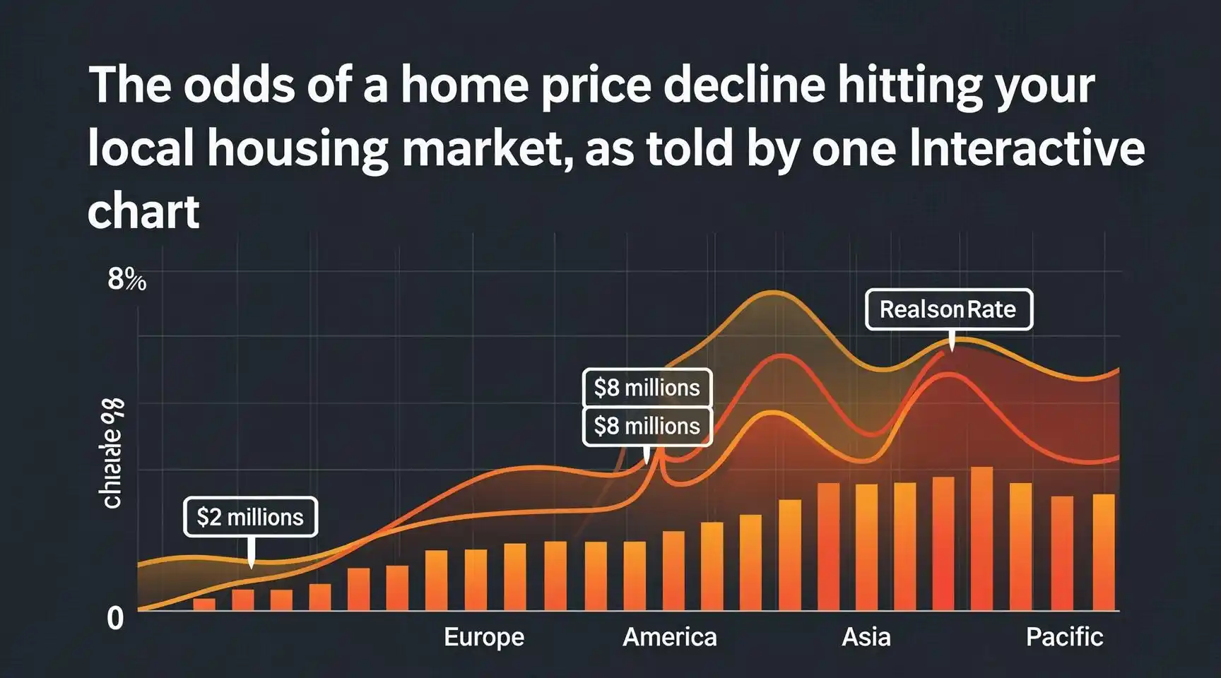
The Comprehensive Analysis: The Odds of a Home Price Decline Hitting Your Local Housing Market, as Told by One Interactive Chart

Step 1: Introduction – The Era of Uncertainty

For years, the housing market has been characterized by a seemingly inexorable rise in values. Homeownership has transformed from a cornerstone of stability into a vehicle for wealth accumulation, driven by a confluence of low interest rates, demographic shifts, and a chronic shortage of inventory. However, as the economic tides turn—marked by fluctuating interest rates, inflationary pressures, and a cooling global economy—the question on every homeowner, buyer, and investor’s lips is the same: Will prices go down?

The answer to this question is rarely found in a national average. Real estate, as the old adage goes, is local. A downturn in San Francisco does not imply a crash in Cleveland, and a stabilization in Austin might not reflect what is happening in Miami. To truly understand the risk to your specific financial future, one must look beyond the headlines and dive into the granular data. This is where the power of data visualization becomes undeniable. By examining a single, comprehensive interactive chart, we can decode the probability of price declines across the nation, transforming abstract economic fears into concrete, actionable intelligence.

This analysis serves as a step-by-step expansion of the insights derived from such a chart, peeling back the layers of the housing market to reveal the hidden risks and opportunities lying beneath the surface.

Step 2: Understanding the Interactive Chart

Before we can interpret the odds, we must understand the tool itself. The interactive chart in question is not merely a static line graph showing median home prices over time. It is a dynamic, multidimensional heat map that overlays various economic indicators to calculate a “risk score” or probability percentage for price declines in specific metropolitan statistical areas (MSAs).

The chart typically functions by allowing the user to hover over or select a specific region, revealing a complex algorithm derived from several key inputs:

1. Price-to-Income Ratios: How expensive homes are relative to what people earn.
2. Inventory Levels: The supply of homes for sale relative to demand.
3. Mortgage Rates: The current cost of borrowing.
4. Migration Patterns: Where people are moving into and leaving from.
5. Employment Growth: The health of the local job market.

When you interact with the chart, you are essentially asking the data: “Given current economic conditions, what is the statistical likelihood that home prices in this specific zip code or city will be lower in 12 months than they are today?” The result is a color-coded landscape of risk, ranging from deep blues (indicating stability or growth) to alarming reds (signaling a high probability of decline).

Step 3: The National Context – A Tale of Two Markets

To understand the local, we must briefly glance at the national. The interactive chart reveals a distinct bifurcation in the American housing market. We are no longer experiencing a monolithic “national housing boom.” Instead, the chart highlights a divergence between “Pandemic Boomtowns” and “Legacy Markets.”

During the pandemic, remote work unlocked a new era of mobility. Workers fled high-cost coastal cities for the spacious, affordable pastures of the Sun Belt and Mountain West. Cities like Boise, Idaho; Austin, Texas; and Phoenix, Arizona saw home values skyrocket at unprecedented rates. The interactive chart shows these regions flashing with higher probabilities of price correction. Why? Because prices rose too far, too fast, often outpacing the actual wage growth of the local population. These markets are currently experiencing a “hangover” as inventory returns and buyers retreat, leading to a natural regression toward the mean.

Conversely, the “Legacy Markets”—established economic powerhouses with strict zoning laws and geographic constraints (such as the San Francisco Bay Area, Boston, and New York)—show different patterns. While affordability is a massive issue there, the inventory constraints are structural, not cyclical. The chart often shows these areas having lower probabilities of severe decline, not because they are booming, but because supply is so tightly controlled that prices have a “stickiness” that prevents free-fall. However, high interest rates can still cause a stagnation in prices, even if a nominal crash is less likely.

Step 4: Decoding the Variables – The Mathematical Drivers of Decline

The interactive chart calculates its odds based on a sophisticated interplay of variables. Let us expand on the specific mechanics that drive these probabilities up or down.

The Impact of Interest Rates: The single most significant lever on the chart is the prevailing mortgage rate. When rates rise from 3% to 7% or higher, purchasing power is decimated. A buyer who could afford a $500,000 home at 3% can only afford roughly $320,000 at 7%. The chart visualizes this shock. In markets where buyers are highly rate-sensitive, the probability of price decline spikes. The chart essentially asks: Can the local income support these prices at these rates? If the answer is no, the risk meter rises.

Inventory Gluts vs. Shortages: The chart tracks “Months of Supply.” A balanced market typically has 4 to 6 months of supply. During the boom, many markets had less than 1 month. As the market cools, inventory rises. The chart highlights areas where inventory is expanding rapidly as high-risk zones. If a market jumps from 1 month to 4 months of supply in a quarter, the probability of a price drop increases exponentially. This is the law of supply and demand in its purest form. When sellers outnumber buyers, prices must fall to clear the market.

The Speculative Index: One of the darker features of such charts is the tracking of investor activity. During the boom, institutional investors and amateur flippers flooded the market. The interactive chart often flags markets with a high percentage of non-owner-occupied homes (rentals and flips) as high risk. When the music stops, speculators are the first to exit. If a market is saturated with investors looking to liquidate portfolios, the chart will show a high probability of a fire sale-driven decline.

Step 5: Regional Deep Dives – What the Map Tells Us

Let’s simulate a journey across the interactive chart to see what specific regions are revealing.

The Southwest (Phoenix, Las Vegas): Hovering over these regions often yields a “high risk” warning. These markets were the epicenter of the pandemic migration wave. Prices rose 40-60% in two years. Now, as remote work policies shift and migration cools, these markets are seeing a surge in listings. The chart shows a “double whammy” of high prices and rising inventory, leading to a mathematical likelihood of price corrections as sellers compete for a shrinking pool of qualified buyers.

The Southeast (Florida, Georgia, the Carolinas): The picture here is mixed. Florida, for instance, saw massive population growth but is now grappling with soaring insurance premiums and climate risk factors. The chart may show a high probability of price declines specifically in coastal, high-risk insurance zones, while inland suburban areas might remain stable. The algorithm is likely factoring in the cost of ownership beyond just the mortgage—specifically insurance and taxes—which are becoming prohibitive.

The Midwest (Columbus, Indianapolis, Kansas City): Here, the chart likely glows with “Stability” or “Low Risk” colors. These markets never saw the absurd price spikes of the coasts. Price-to-income ratios remain reasonable. While they are not immune to national interest rate trends, the underlying fundamentals are sound. The probability of a massive price crash here is low because there was no massive bubble to pop. The chart suggests these markets may see a flattening of prices rather than a decline.

The West Coast (Seattle, Portland, California): This is the “Correction without Crash” zone. The chart may show a moderate risk of decline. Prices are so astronomically high that even a small drop in demand forces sellers to lower asking prices. However, because new construction is nearly impossible due to regulation and geography, the supply never truly floods the market. The chart likely predicts a slow bleed (nominal declines) or a period of stagnation where prices drift sideways for years.

Step 6: The Psychology of the Market – Fear and the Feedback Loop

Charts and data are objective, but markets are driven by human emotion, which is subjective. The interactive chart is a lagging indicator of hard data, but it also attempts to predict future sentiment.

When users look at this chart and see their city painted red (high probability of decline), a psychological feedback loop begins. Potential buyers see the data and decide to “wait for the bottom.” This reduction in demand creates the very decline the chart predicted. Conversely, in areas painted green (low probability), buyers feel a sense of urgency (FOMO), driving prices up and validating the chart’s prediction.

The chart effectively gamifies the housing market. It quantifies “Fear, Uncertainty, and Doubt” (FUD). Understanding this psychological component is crucial. If the chart says there is a 60% chance of a decline in your neighborhood, it is not just a prediction; it becomes a self-fulfilling prophecy as market participants react to the risk.

Step 7: Time Horizons – Short Term Pain vs. Long Term Gain

A critical step in expanding this analysis is defining the timeframe. The interactive chart usually offers probabilities for a 1-year or 2-year horizon. It is vital to distinguish between a “cyclical correction” and a “permanent loss of value.”

A 10% to 20% drop in home prices over two years can feel catastrophic for a seller, but on a 10-year timeline, it may appear as a minor blip. The chart helps investors distinguish between markets that are merely taking a breath and those that are facing structural collapse.

For example, a market dependent on a single industry (like a tech hub or a manufacturing town) faces structural risk if that industry struggles. The chart will show a persistently high probability of decline over multiple years. In contrast, a diversified economy might show a short-term spike in risk probability (due to high rates) but a quick return to stability. The interactive tool allows users to toggle these timeframes, revealing that the “odds of a decline” are not static; they change as the economic cycle progresses.

Step 8: What the Data Means for You – Strategic Implications

For the Homeowner: If the chart shows a high probability of decline in your area, it does not necessarily mean you should sell immediately. Transaction costs (real estate commissions, closing costs, taxes) often eat up 10% of a home’s value. If the chart predicts a 5% decline, selling is a losing proposition. However, if you were planning on downsizing or moving anyway, the chart serves as a warning to list your home now, before the anticipated decline materializes further.

For the Buyer: The chart is a treasure map for opportunity. Areas with a high probability of decline are “watch list” items. If you can wait, you might secure a property for significantly less in 12 to 18 months. However, you must balance this against the cost of renting and the potential for interest rates to drop (which would spike demand and prices back up). The chart helps you time the market, but it cannot time the Federal Reserve.

For the Investor: This is your risk management tool. The interactive chart helps you avoid “catching a falling knife.” By identifying markets with a high probability of decline, you can steer your capital toward “defensive” assets—markets with low probability of decline and high rental yields. The chart confirms that the era of “anything goes” speculation is over; the new era requires surgical precision based on data.

Step 9: The Limitations of the Model

No chart is a crystal ball. While this interactive tool is powerful, it has limitations. It relies on historical data to predict future outcomes. It cannot account for “Black Swan” events—a sudden geopolitical crisis, a massive change in immigration policy, or a technological breakthrough that revitalizes a dying city.

Furthermore, real estate data is often reported with a lag. The “closed sales” data the chart uses reflects contracts signed 30 to 60 days ago. In a fast-moving market, the chart might be telling you what happened two months ago, not what is happening today. Savvy users must combine the chart’s historical data with real-time anecdotal evidence—talking to local agents, watching open house traffic, and monitoring pending sales.

Step 10: Conclusion – Navigating the New Normal

The odds of a home price decline hitting your local market are no longer a matter of guesswork. Through the lens of this interactive chart, we can see that the housing market is fracturing. The uniform red-hot heat of the pandemic era has cooled, leaving a patchwork of temperatures across the nation.

The chart tells a story of normalization. Prices that detached from reality are gravity-bound. Markets that grew sustainably are weathering the storm. For anyone with a stake in real estate, the takeaway is clear: Ignore the national averages. Dive into the local data. Understand the specific economic DNA of your zip code.

Whether you are buying, selling, or holding, the interactive chart provides the probabilities you need to make informed decisions. It removes the emotion from the equation and replaces it with evidence. In a market defined by uncertainty, that is the most valuable asset of all. The probability of a decline is real in many areas, but with the right data, you can navigate the downturn and position yourself for the eventual recovery.

Keywords

1. Real Estate Forecast
2. Housing Market Correction
3. Local Market Analysis

Hashtags

#RealEstate #HousingMarket #Economy

Disclaimer

The content provided in this analysis is for informational and educational purposes only. It is based on general data trends and hypothetical interactive chart interpretations and does not constitute financial, investment, or legal advice. Real estate markets are inherently volatile and subject to rapid changes. All readers are encouraged to consult with qualified financial advisors, real estate professionals, and accountants before making any property-related decisions. The author and publisher assume no responsibility for any actions taken based on the information provided herein.